In 2014, Jane Street Jane Street has been publishing monthly puzzles for a while now. Broadly speaking, they fall into one of three categories: riddles (look for clues), mathematical problems (reason and calculate), and computational problems (write a fast program). While it certainly can be solved by hand – placing it in the mathematical category – the subsequent ‘Hooks’ puzzles become infeasible without the help of a computer. Moreover, I really want to talk about SMT solvers, so we’ll start ‘programming’ right from the beginning! published the following puzzle:

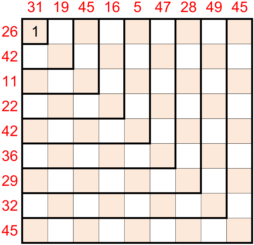
In the grid below, enter nine 9’s in the outermost hook, eight 8’s in the next hook, then seven 7’s, six 6’s, and so on, down to the one 1 (already entered), so that the row and column sums match the values given along the border.

Once you’ve completed the puzzle, submit as your answer the sum of the values of the shaded squares.

Without much actual programming, we will magically obtain a solution. Keyword: SMT solvers. The full code is available here.

Motivation

When I first started using Lean, I learned that it is a proof assistant and not an automated theorem prover. Knowing neither, I looked into both, and – to add to the confusion – discovered that one of Lean’s primary authors also helped develop a famous automated theorem prover, Z3! I had a lot of fun experimenting with it, but since I needed to finish my thesis, I set it aside for a while. Recently, at the Dutch Formal Methods Day, I met Marijn Heule, one of the editors of the Handbook of Satisfiability. Talking to him inspired me to take a second look.

Background

DISCLAIMER: This section merely serves as an introduction to SAT and SMT; don’t expect full mathematical rigor.

Let’s start with the basics: the boolean satisfiability problem, or SAT for short. Any mathematician/computer scientist will – or at least should – learn about this. SAT is the decision problem of determining whether a given boolean formula is satisfiable, that is, if there exists some interpretation of the variables (a model) such that the formula evaluates to TRUE.

An example should clarify this further. Say the formula you’re interested in is p ∧ ¬q (p and not q). Then setting p = TRUE and q = FALSE guarantees that the formula holds, hence it is satisfiable. The model we used here is {p = TRUE; q = FALSE}.

The theoretical importance of SAT stems from the fact that it was the first – not completely obvious – problem that was shown to be NP-complete. This result is known as the Cook-Levin Theorem. If you’re interested in the NP-completeness of other problems, it now suffices to show that the new problem is in NP and that SAT reduces to it. In particular, you no longer need to work directly with Turing machines. For some time, I wrongly assumed that this meant SAT has no practical use. However, although a general efficient algorithm might not exist, Even if P = NP, it seems unlikely a reasonable polynomial-time algorithm exists. it is still extremely valuable to implement such SAT solvers since so many real-world problems can be encoded into it, and, as it turns out, these solvers are very efficient in practice. Donald Knuth has a section (Section 7.2.2.2) about it in The Art of Computer Programming, almost 300 pages long, and stated the following in Fascicle 6 of Volume 4:

The SAT problem is evidently a killer app, because it is key to the solution of so many other problems. […] The story of satisfiability is the tale of a triumph of software engineering, blended with rich doses of beautiful mathematics. Thanks to elegant new data structures and other techniques, modern SAT solvers are able to deal routinely with practical problems that involve many thousands of variables, although such problems were regarded as hopeless just a few years ago.

Applications include scheduling problems, software and hardware verification, and of course silly puzzles!

But you may still be wondering: what exactly is SMT then? This stands for satisfiability modulo theories. Just as SAT is the decision problem of determining the satisfiability of formulas in propositional logic, SMT extends this to first-order logic with respect to a background theory, What if one writes a general-purpose solver for first-order logic, you ask? For one, this is a more generic problem, and therefore harder to optimize. Moreover, the fixed interpretation requires us to add additional formulas which the model should satisfy. However, some theories cannot be described by a finite set of first-order formulas (finite trees), or even a decidable set (integer arithmetic)! SMT solvers overcome this hurdle, at the cost of being restricted to a particular domain. See the Handbook of Satisfiability, Chapter 33. which fixes the interpretation of certain predicate and function symbols. For our puzzle, we’ll work in the theory of integer arithmetic. Fixing the interpretation simply means that if our formula uses symbols such as +, 0 or 1, they should have the usual interpretation of addition, zero or one in integer arithmetic.

Again, an example should hopefully clarify this. Suppose the formula we are interested in is x + 1 = 1. If we set x = 0, this formula holds, with the usual interpretation of the symbols of integer arithmetic. Intuitively, our model now is {x = 0; <all of integer arithmetic>}. What we absolutely do not want is a model where, for example, every integer symbol is interpreted as the same element, and + is the binary function that maps everything to this element. In this model, the formula is also satisfied – regardless of the interpretation of x – but clearly, that is not what we’re after.

Translating the problem

Our next subgoal will be to somehow reduce the puzzle to a formula in the theory of integer arithmetic such that a model satisfying the formula leads to a solution of the puzzle. The variable x_i, j will represent the value of the cell in row i and column j of the grid. There are four kinds of constraints that our solution should satisfy:

a cell should be empty or contain the value of the hook it is in
the n-th hook should contain precisely n non-empty cells
the cells in a row have a prescribed sum
the cells in a column have a prescribed sum

The first question is how to encode empty cells. Since the last two constraints use sums, and empty cells should not affect this sum, it is natural to let empty cells correspond to 0. Once we fix these possibilities for a cell’s value, the hook constraint is equivalent to:

the cells in the n-th hook sum to n ⋅ n

This yields the following constraint formulas:

Cell constraints:
x_1, 1 = 1 or x_1, 1 = 0
x_1, 2 = 2 or x_1, 2 = 0
⋮
x_9, 9 = 9 or x_9, 9 = 0
Hook constraints:
x_1, 1 = 1
x_2, 1 + x_2, 2 + x_1, 2 = 4
⋮
x_9, 1 + x_9, 2 + … + x_9, 9 + … + x_2, 9 + x_1, 9 = 81
Row constraints:
x_1, 1 + x_1, 2 + … + x_1, 9 = 26
x_2, 1 + x_2, 2 + … + x_2, 9 = 42
⋮
x_9, 1 + x_9, 2 + … + x_9, 9 = 45
Column constraints:
x_1, 1 + x_2, 1 + … + x_9, 1 = 31
x_1, 2 + x_2, 2 + … + x_9, 2 = 19
⋮
x_1, 9 + x_2, 9 + … + x_9, 9 = 45

The actual formula the model should satisfy is then simply the conjunction of all the ones above. If such a model miraculously appears, the answer to the puzzle can be calculated as

x_1, 1 + x_1, 3 + x_1, 5 + … + x_9, 9.

The actual solution

What remains is actually finding a suitable model. We’ll use the SMT solver Z3 for this. It provides bindings for various programming languages, but we’ll stick to Python. This will serve as a kind of meta-language to construct the formula we described in the previous section – I really don’t want to write it by hand. There are many well-written tutorials on using Z3 with Python available online, There is an official tutorial, but perhaps also look at this gentle introduction, or read this broad, yet practical overview. but the code should be self-explanatory if you’ve been able to follow so far.

from z3 import *

rows = [ 26, 42, 11, 22, 42, 36, 29, 32, 45 ]
cols = [ 31, 19, 45, 16,  5, 47, 28, 49, 45 ]

 # Create a 9x9 grid of integer variables.
X = [[Int("x_%s_%s" % (i + 1, j + 1)) for j in range(9)] for i in range(9)]

cell_constraints = [
    Or(X[i][j] == max(i + 1, j + 1), X[i][j] == 0) for i in range(9) for j in range(9)
]

hook_constraints = [
    Sum([X[i][n] for i in range(n + 1)] + [X[n][i] for i in range(n)])
    == (n + 1) * (n + 1)
    for n in range(9)
]

row_constraints = [Sum(X[i]) == rows[i] for i in range(9)]

column_constraints = [Sum([X[i][j] for i in range(9)]) == cols[j] for j in range(9)]

# The problem is simply a list of constraints.
problem = cell_constraints + hook_constraints + row_constraints + column_constraints

# Here is where the magic happens.
solver = Solver()
solver.add(problem)
solver.check()
model = solver.model()

# Extract the grid from the obtained model.
grid = [[model.evaluate(X[i][j]).as_long() for j in range(9)] for i in range(9)]
print("The correct grid is:")
print_matrix(grid)

# Calculate the actual answer.
answer = sum([grid[i][j] for j in range(9) for i in range(9) if (i + j) % 2 == 0])
print(f"The final answer is {answer}.")

Running Make sure you have Z3’s Python bindings installed, for example by using a nix shell, or executing pip install z3-solver – if you want to pollute your global python environment. this with Python yields:

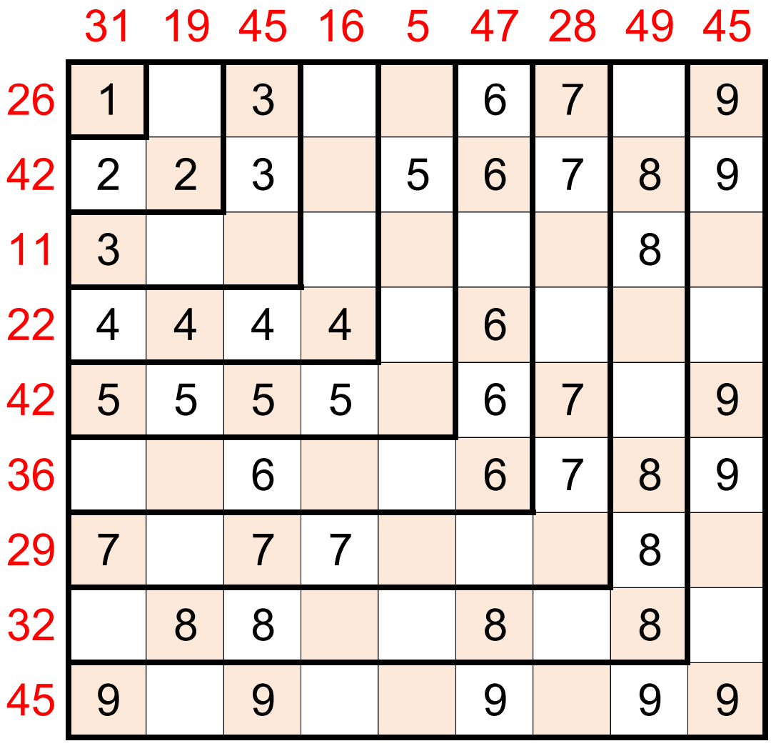
The correct grid is:
[[1, 0, 3, 0, 0, 6, 7, 0, 9],
 [2, 2, 3, 0, 5, 6, 7, 8, 9],
 [3, 0, 0, 0, 0, 0, 0, 8, 0],
 [4, 4, 4, 4, 0, 6, 0, 0, 0],
 [5, 5, 5, 5, 0, 6, 7, 0, 9],
 [0, 0, 6, 0, 0, 6, 7, 8, 9],
 [7, 0, 7, 7, 0, 0, 0, 8, 0],
 [0, 8, 8, 0, 0, 8, 0, 8, 0],
 [9, 0, 9, 0, 0, 9, 0, 9, 9]]
The final answer is 158.

Congratulations on reading all the way to the end! This is indeed the correct solution:

Cracking Jane Street's Puzzles with SMT Solvers: Part 1

Motivation

Background

Translating the problem

The actual solution